I blogged here, arguing that Indian businesses face a structural cost constraint similar to that of developed economies that erode their global competitiveness. This cost constraint on the supply side must be seen alongside a constraint of a consumption class that is far smaller and shallower than imagined. In other words, a developed country's cost structure in a low-income country's market size.
This point has been a consistent argument of this blog and was documented in great detail in Can India Grow? in 2016, much before it became more widely recognised.
India’s demand-side problem is twofold. For a start, it already has a low per capita income, the lowest among its emerging market peers. Second, this itself conceals a low base of the consumption class that is also not widening proportionately with economic growth. The nature of economic growth is such that it is not only not broad-based enough but is also widening inequality.
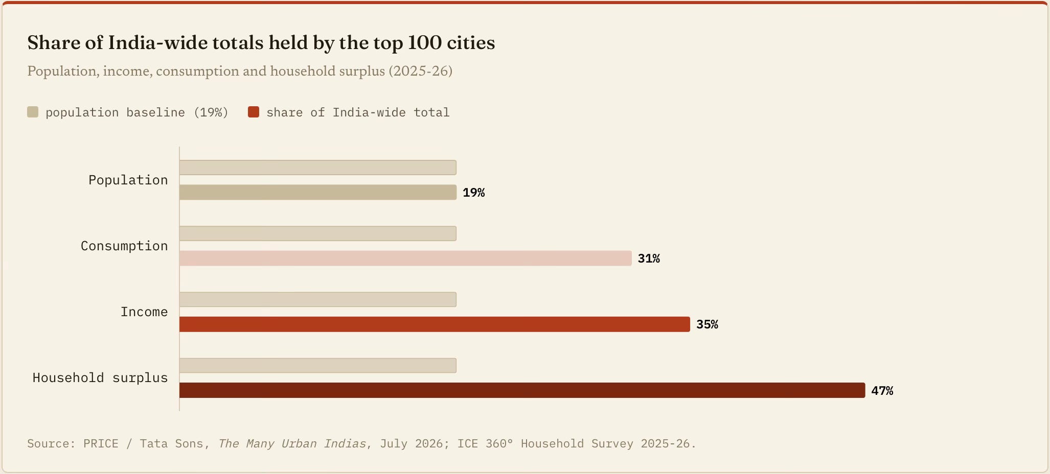
The recently released PRICE - Tata Sons Many Urban Indias report is a confirmation of the demand-side constraint. It finds that the top 100 cities, with just under a fifth of the population, capture almost half of all household surplus, the closest measure to genuine discretionary spending capacity. What sits outside, the other 81% of India, holds only about 53% of surplus combined, and most of that is in the top slices of tier-2/3 towns and the productive rural belt. The surplus-generating layer of the economy is essentially urban and already fully contained. There is no large pool of "middle India" outside urban India waiting to broaden the base.
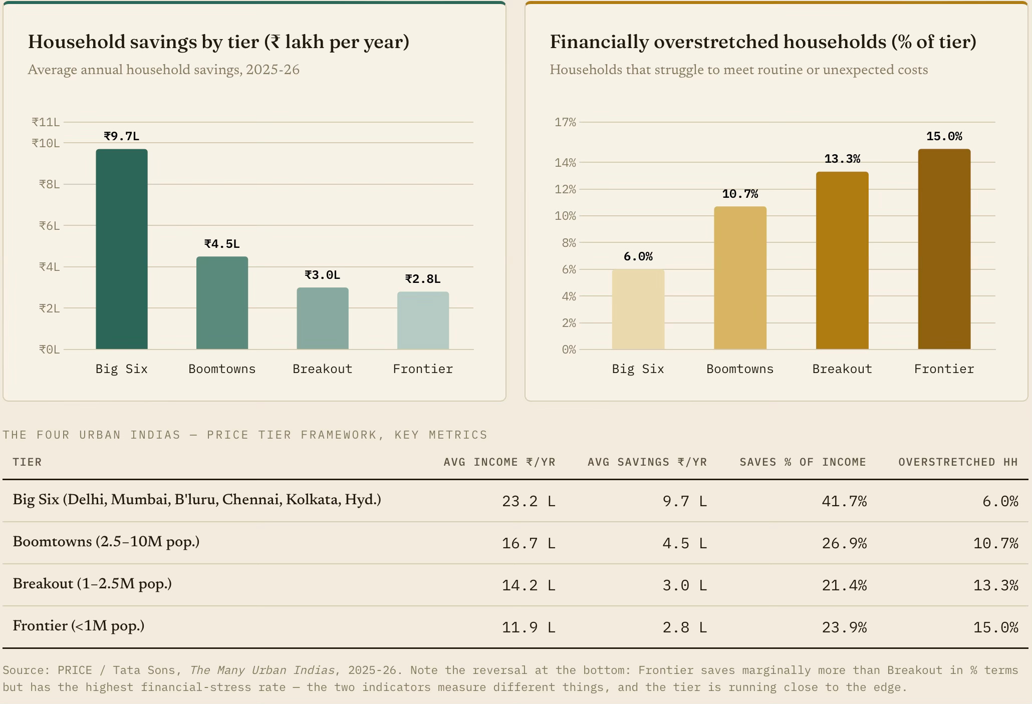
PRICE's top-100 city-tier framework (Big Six, Boomtowns, Breakout, Frontier) is the empirical proof that "urban India" is not a homogeneous consuming class. The gap in savings between the top and bottom tiers is nearly 3.5×, and one in six Frontier-city households is already financially overstretched. This is what “narrow” looks like at the city level.
The top 15 cities have two-thirds of all top-100 consumption, and the Delhi NCR alone has 15% of all urban consumption. The consuming class is a stratum within the Big Six, not the Big Six themselves. Even within the six megacities, PRICE reports that 24% of households are low-income. The consuming class is not "urban India" (~500M) or even "top-100 city India" (282M), but a stratum of prosperous households scattered across the Big Six and the top of the Boomtown tier.
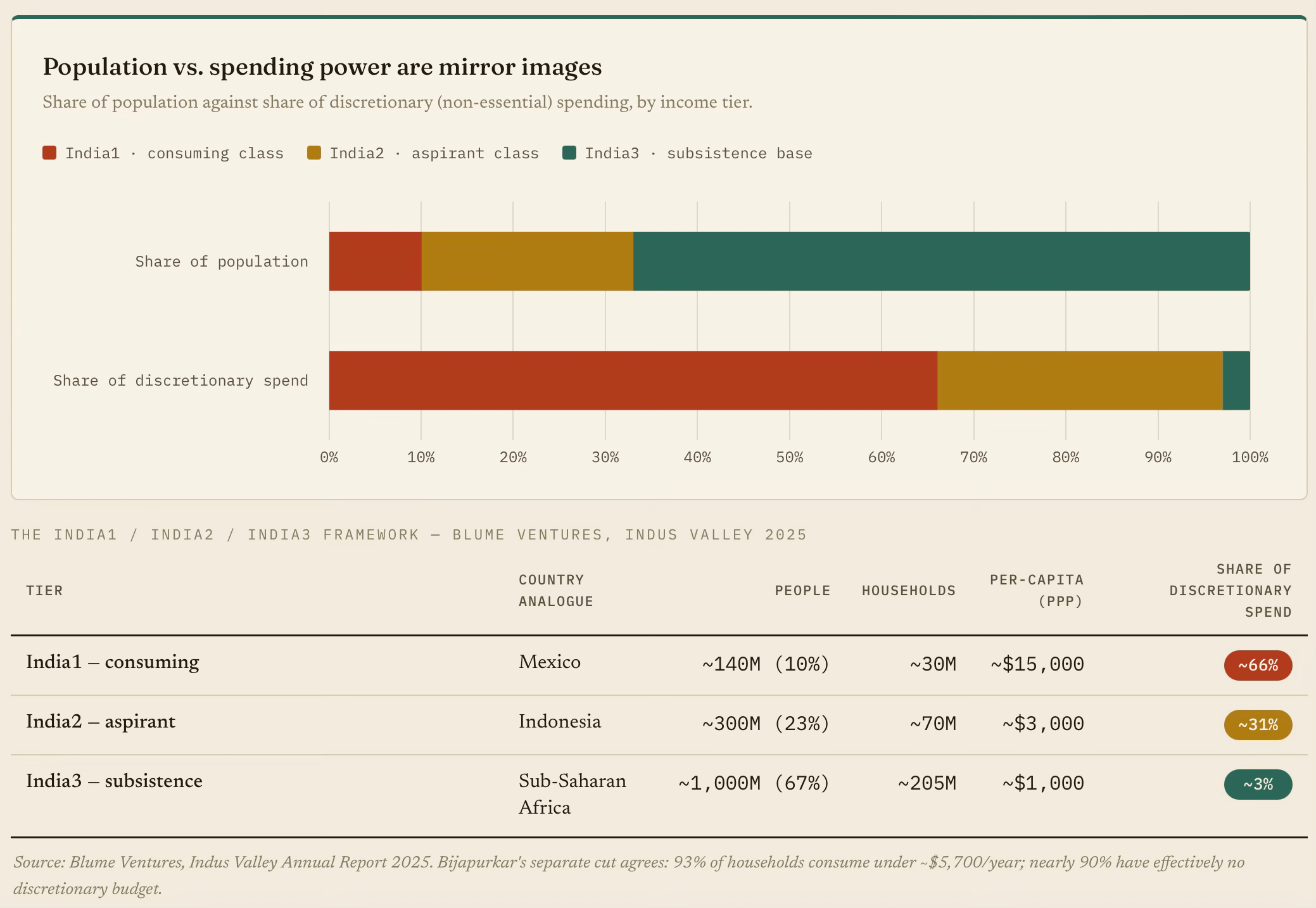
The Blume Ventures categorisation of India’s consumption class finds three groups, with the first comparable in size to the population of Mexico at 30 million households (the Blume Rule of 30, or 10% of Indian households). A worrying finding is that the consuming class that anchors private demand is small and getting deeper, not significantly wider. A vast base has almost no discretionary spending power at all. This is the inverse of the broad, upwardly mobile middle that sustains private investment.
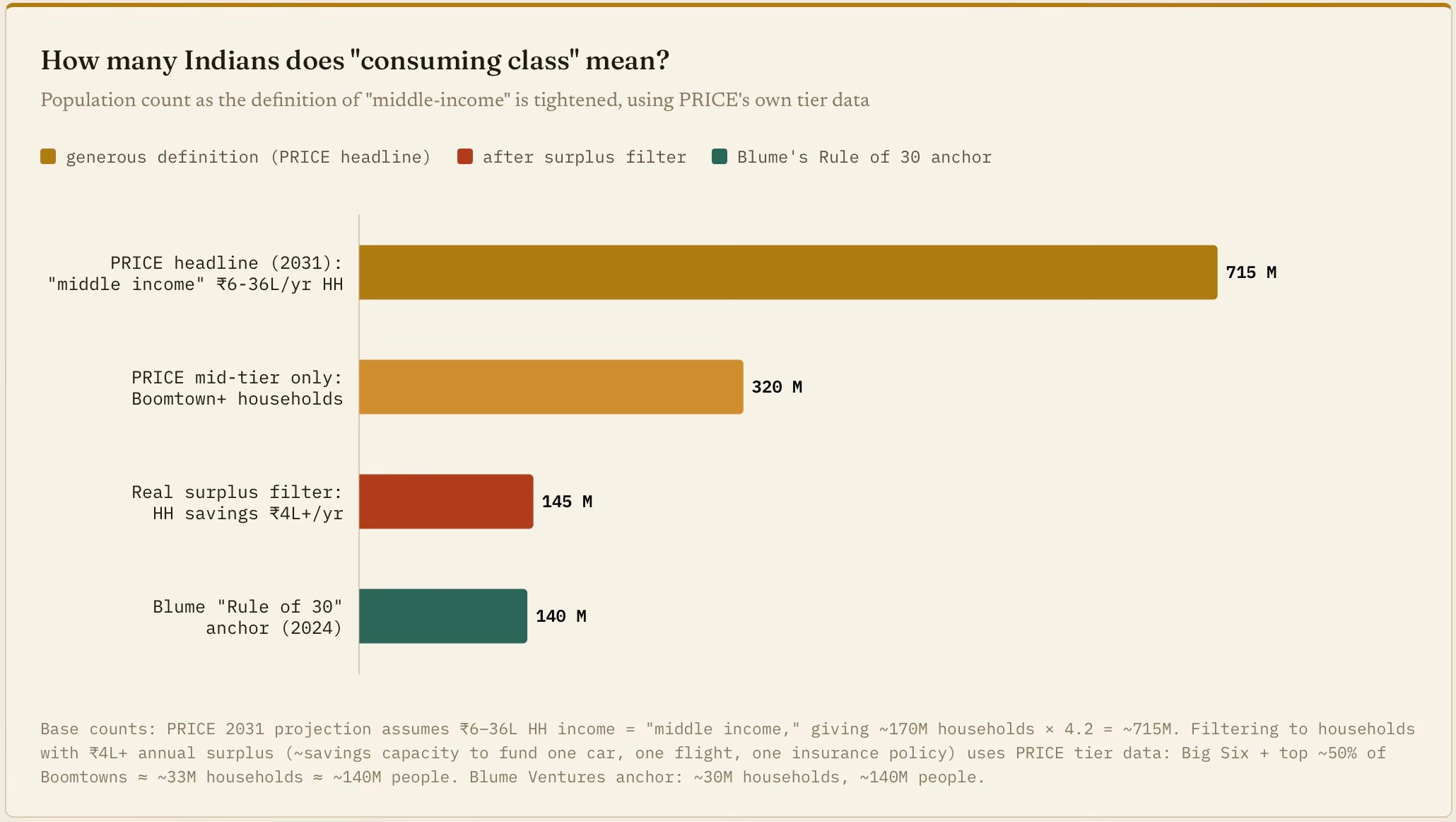
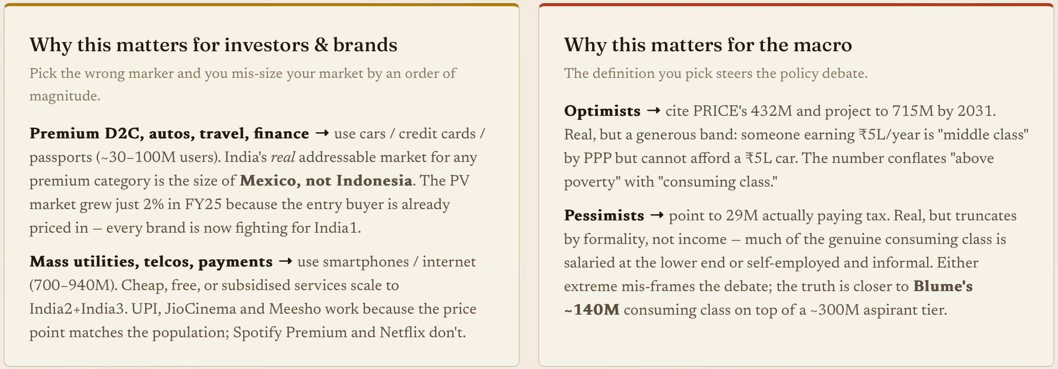
The PRICE report's optimistic headline (~715M "middle income" people by 2031) conflates a household that shares a scooter with one that services a car EMI. Once you apply a real surplus filter - savings above ₹4 lakh a year, which is roughly what it takes to run a car, insure a family, and take one flight - the number lands where Blume said it did. In simple terms, PRICE's 715M by 2031 measures how many Indians will earn enough not to be poor, a significant achievement. Blume's 140M measures how many can act as a consuming class today - the market a brand can actually sell a car, an AC, a holiday abroad or a health-insurance policy to.
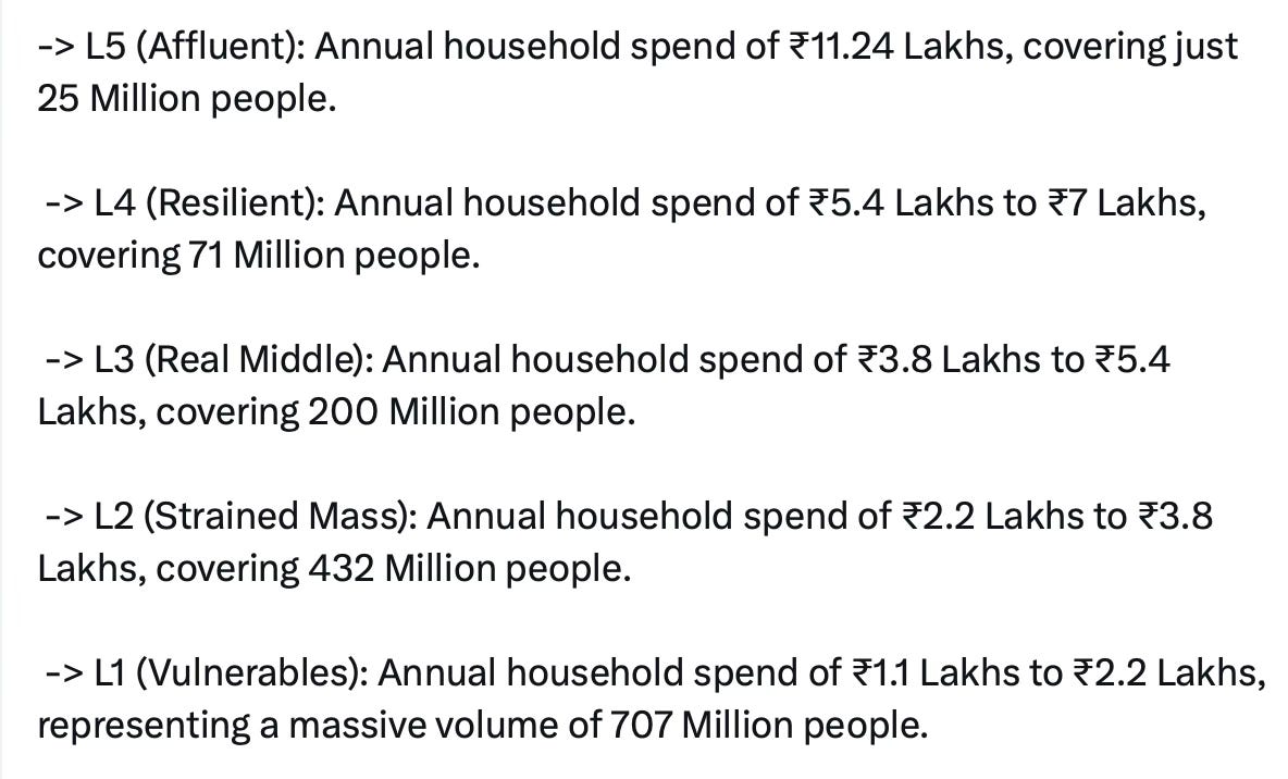
The numbers are further validated by other sources. An income assessment by Rama Bijapurkar points to a more differentiated group, but a similar narrow base of the consumption class. She estimates that 93% of households have annual consumption of less than $5,700.
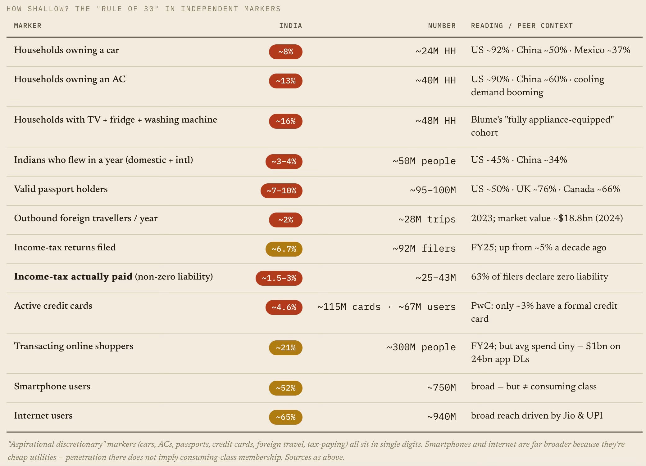
The data on penetration of discretionary goods and behaviours corroborates the Blume survey data. Almost every independent marker lands near the same Blume Rule of 30. Whether you measure cars, ACs, credit cards, foreign travel, or who actually pays income tax, the consuming class converges on the same narrow apex. If anything, the Blume data itself looks too optimistic.
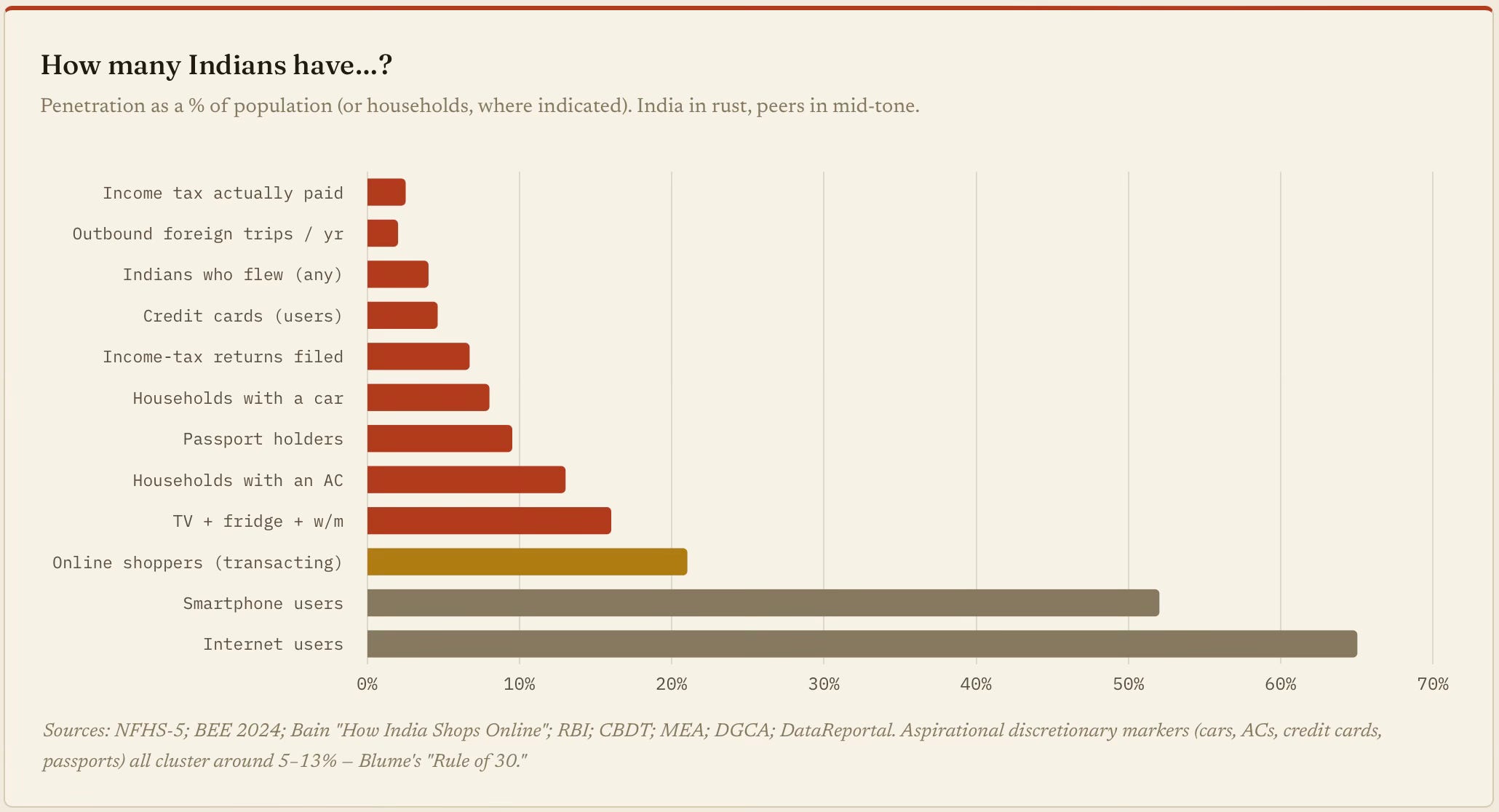
Whichever marker you pick - cars (8%), ACs (13%), passports (~10%), income-tax payers (1.5–3%), credit cards (4.6%), foreign trips (2%) - the consuming class lands at ~10% of households or fewer. That is also exactly where the bottom-up Blume spending model, income surveys of Bijapurkar, and asset penetration estimates of NFHS/Bain lands.
India's "middle class" has been estimated at 29 million people one way and 600 million another, a multiple spread of 20 that reflects what one is choosing to count.
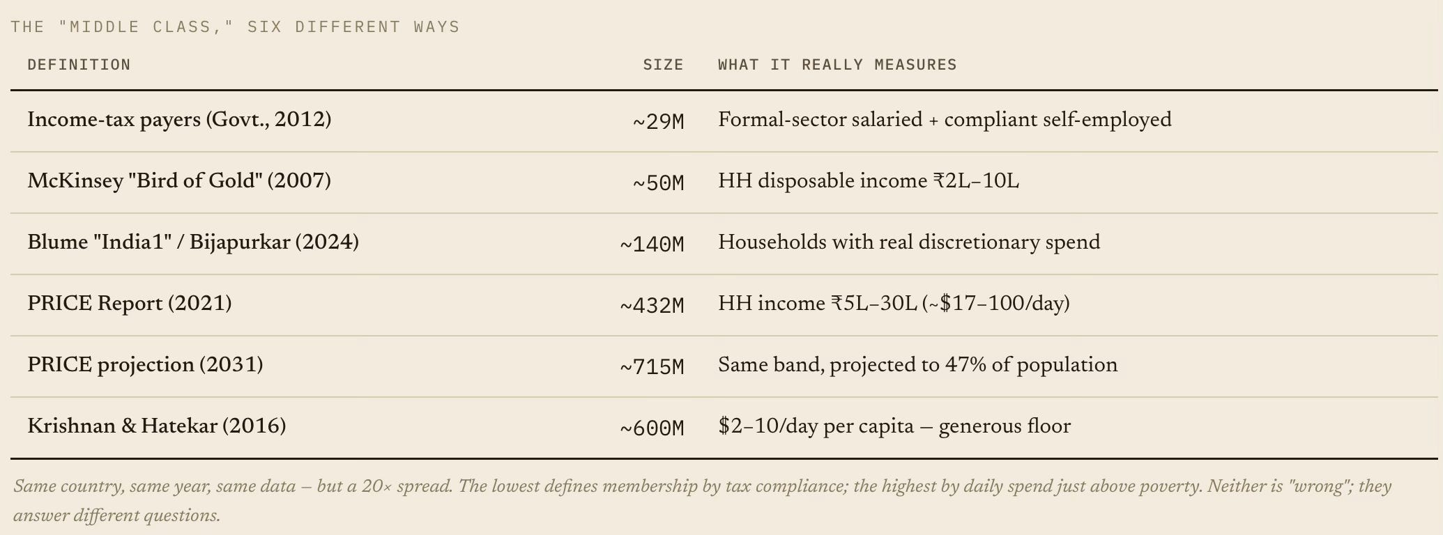
India has a consuming class of ~140M, an aspirant class of ~300M moving toward it, and a base of ~1bn for whom the "middle class" debate is moot. That picture is consistent with every methodology once you ask which question each one answers - how many can afford a car (~10%), how many are above poverty by global standards (~30%), how many participate in the digital economy (~65%). Conflating them is the single most common error in India market-sizing. This is a very nice summary of why nobody gets the elephant in full.
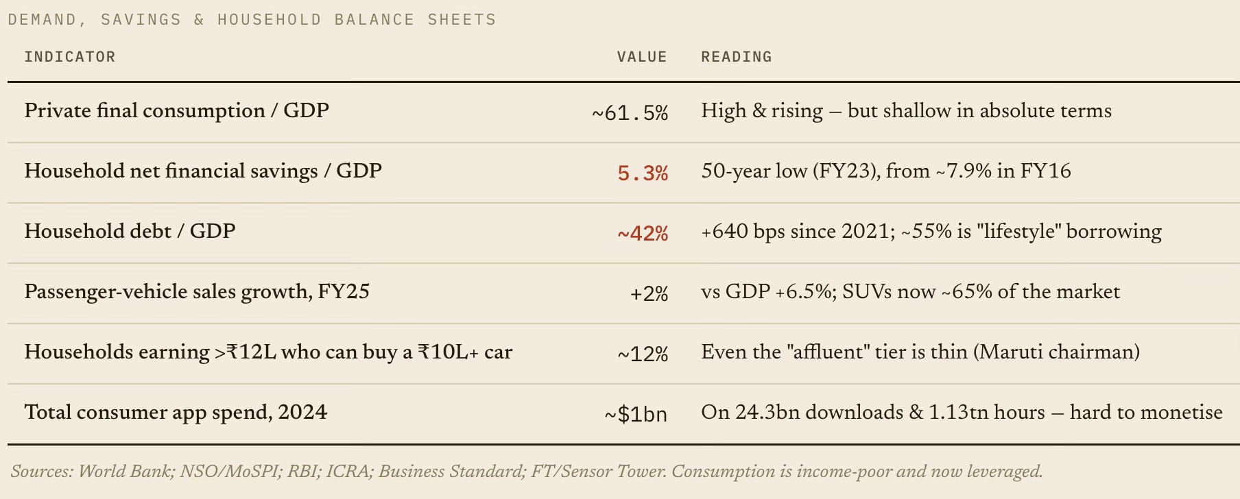
In this context, it is also useful to draw a nuance on India’s high consumption rate of 61% of GDP, which is far higher than China’s ~38% of GDP. India’s problem is that while it is already a consumption-led economy, the problem is the quality of that demand. It is too thin per person, skewed to the top decile, and increasingly financed by debt as households run down savings. In other words, the demand side constraint is not the consumption share of GDP, but that there are too few middle-income earners to generate broad, income-financed volume. That points policy at jobs, wages and investment, not at “stimulating consumption.”
Fundamentally, all the above is a reflection of two important factors - the low per-capita income and the widening inequality in sharing the benefits of aggregate growth.
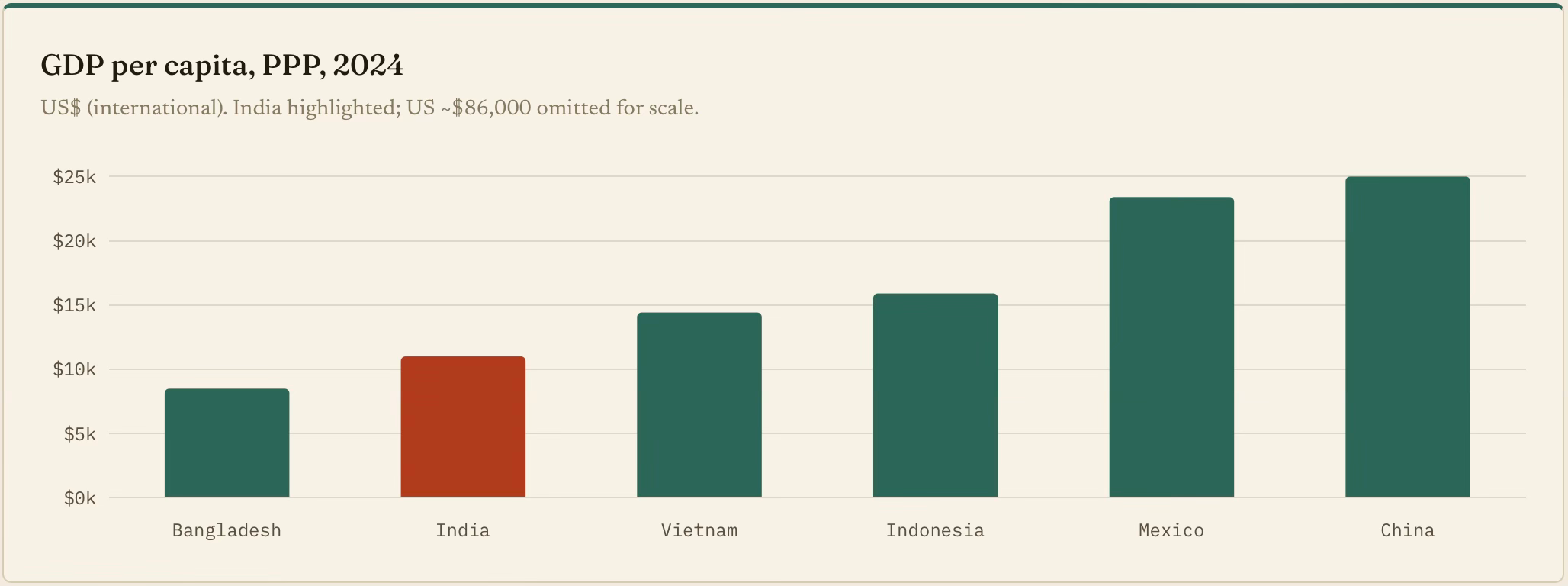
India's per-capita output (PPP) trails Vietnam and Indonesia and is under half of China's. Its Mexico-like consuming tier is real, but at best, only ~10% of the country.
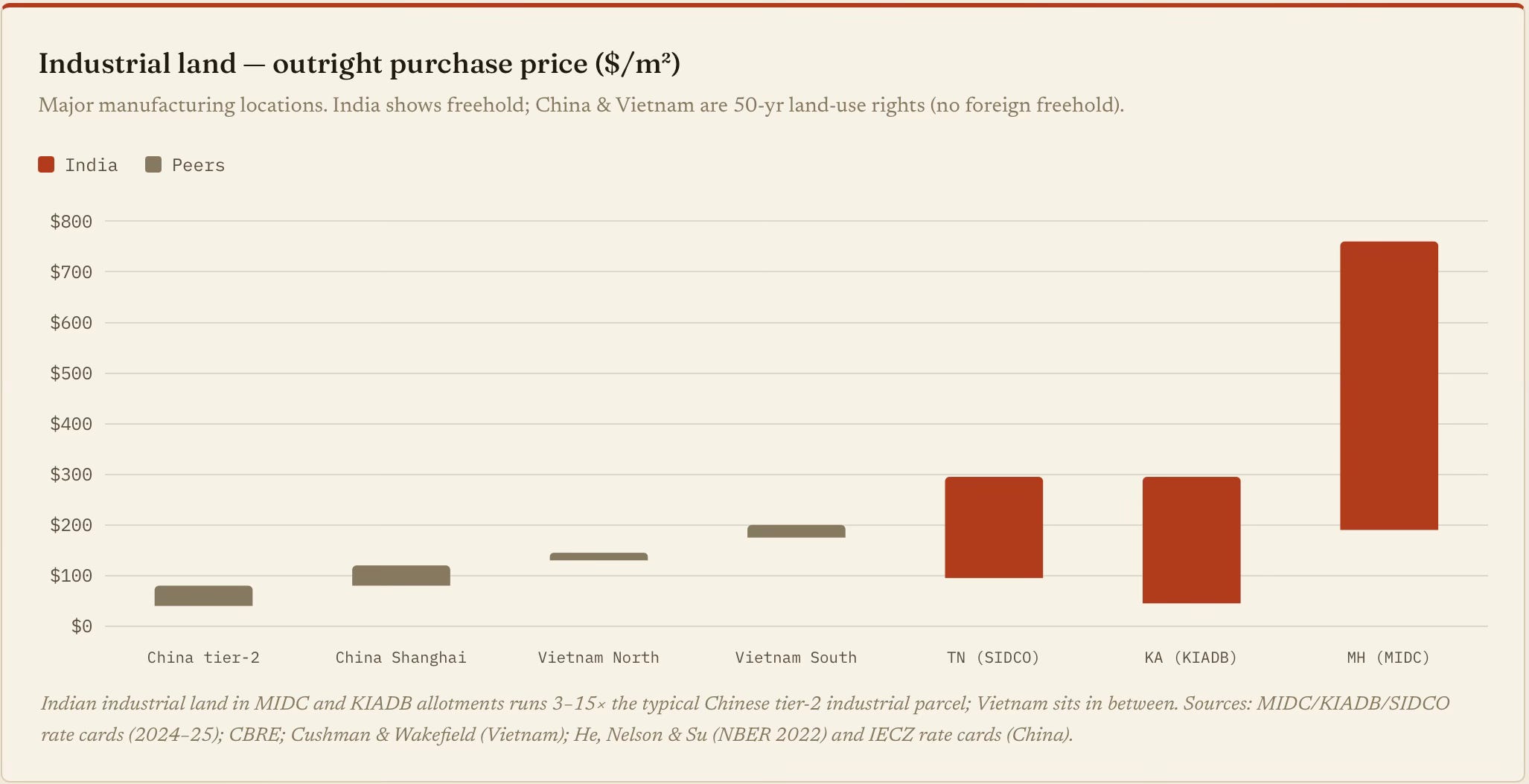
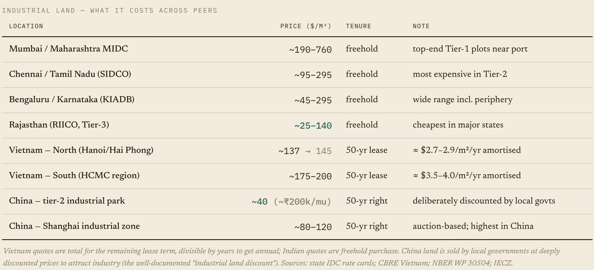
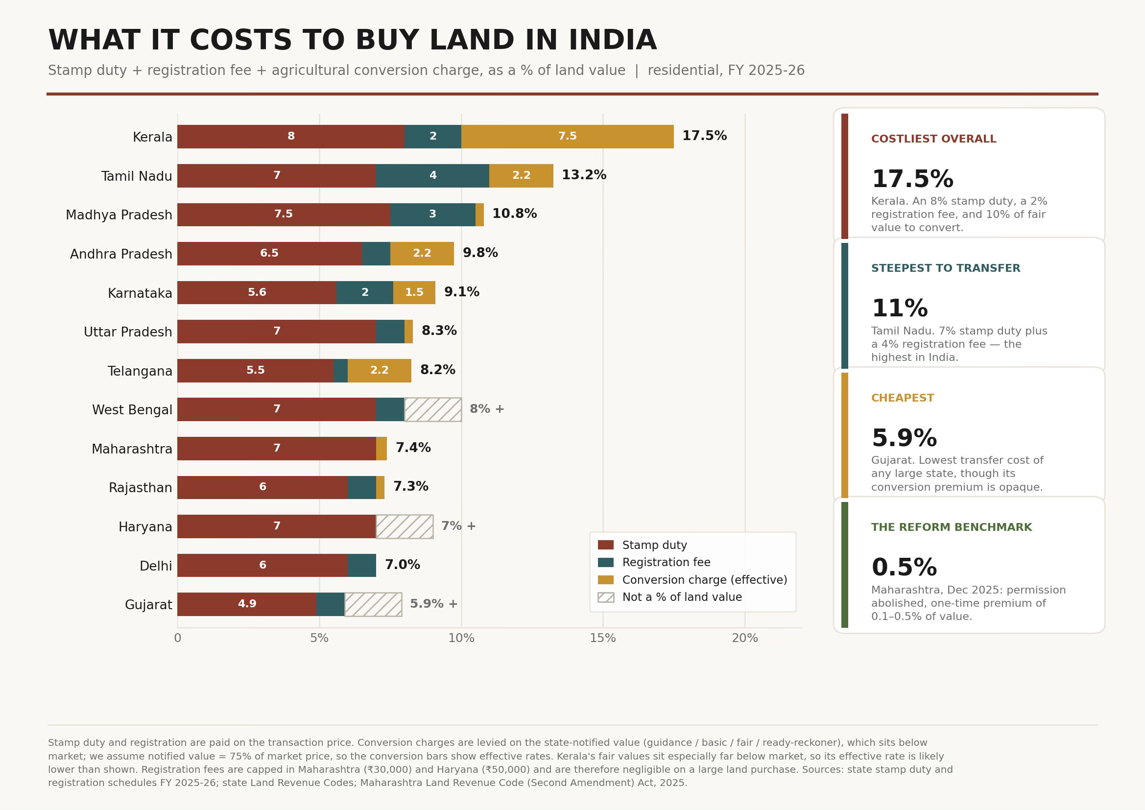
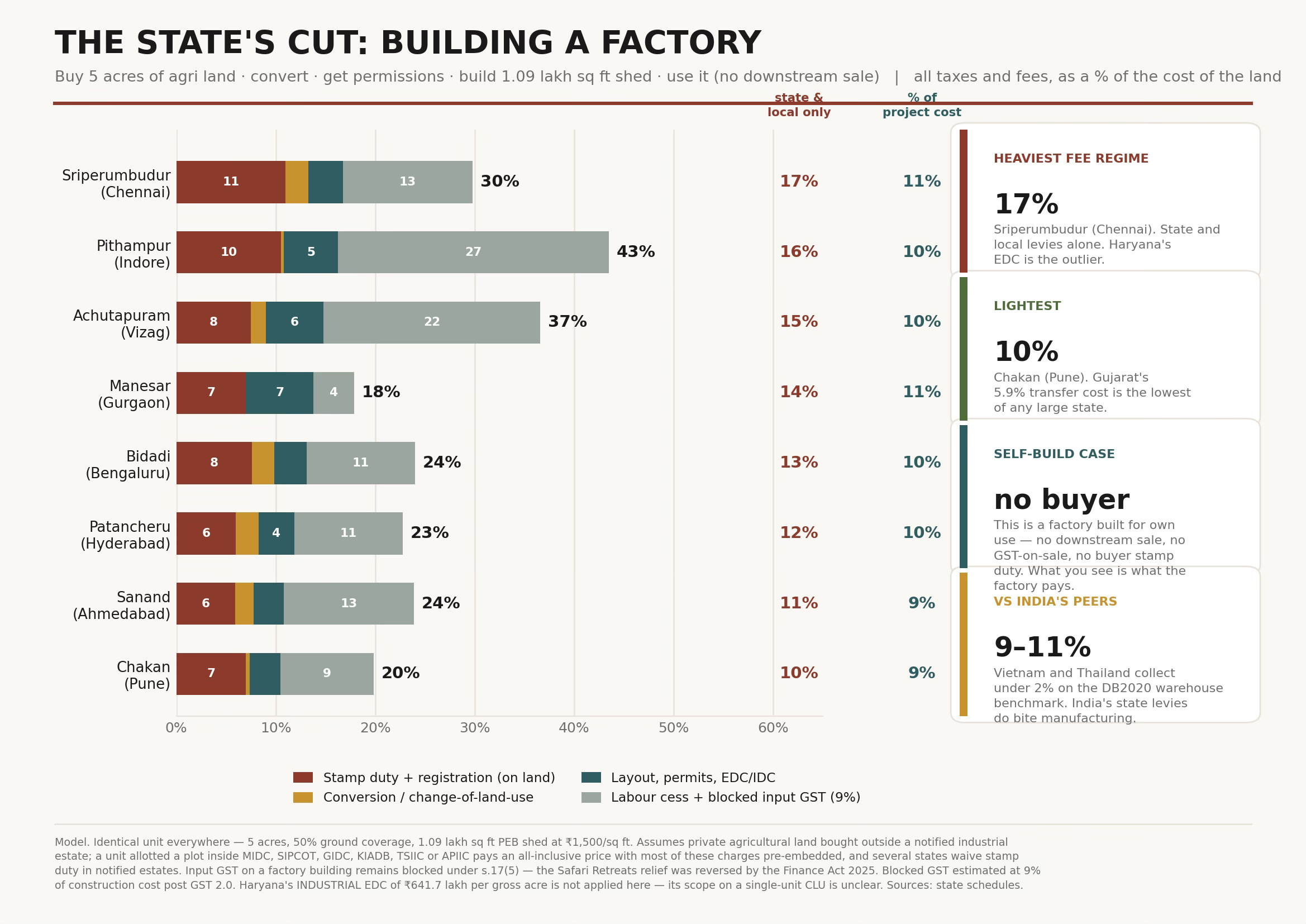
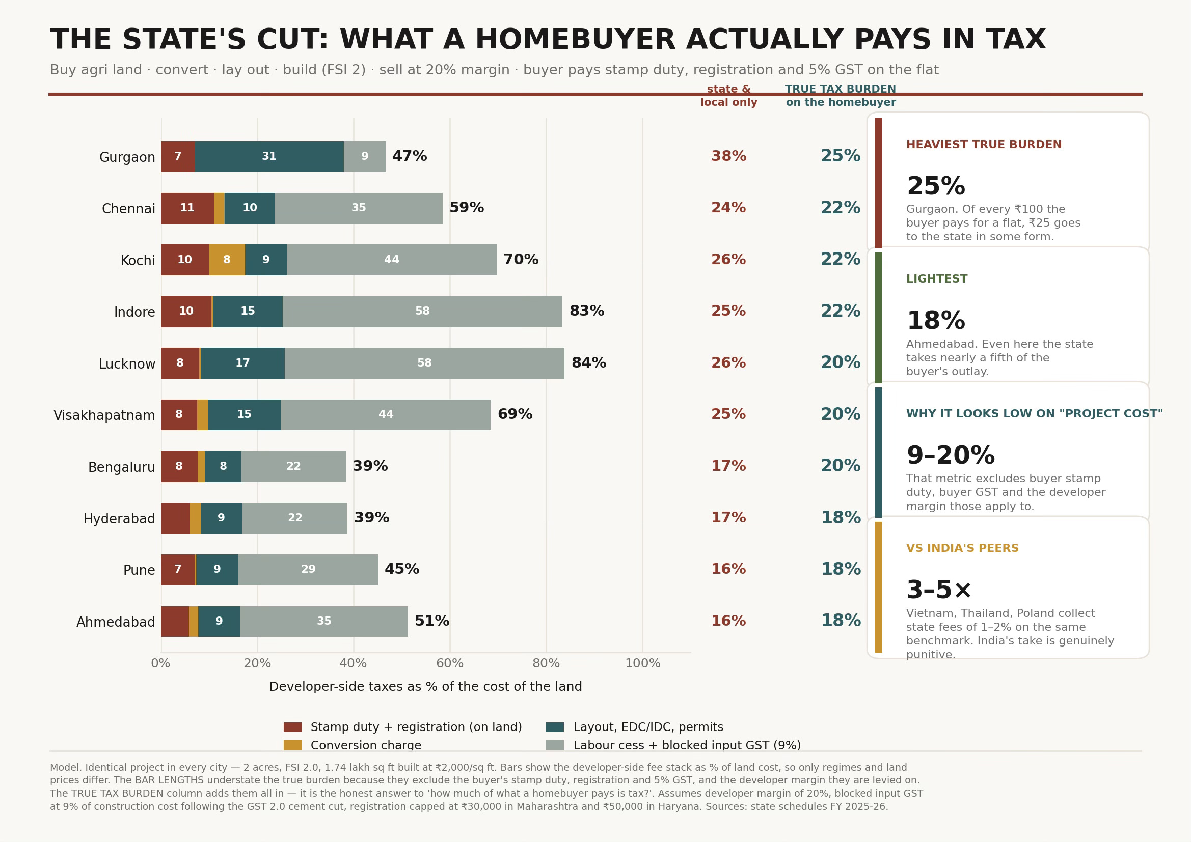
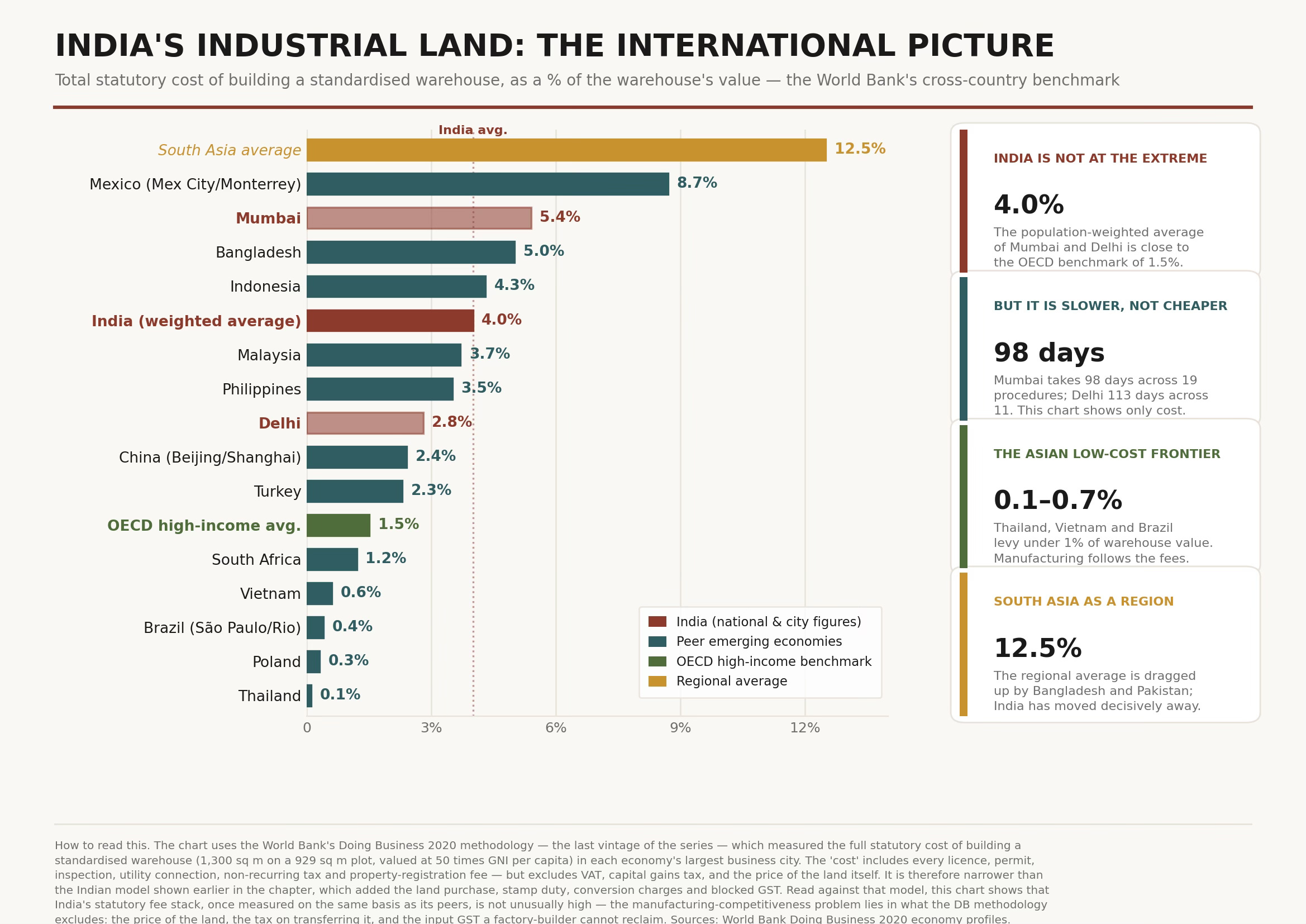
India imposes rich-country costs on poor-country incomes in capital, fuel and land - and because those costs are policy-made, they are the actionable half of the problem. The demand blade can only be widened the slow way: through jobs, wages and productivity.
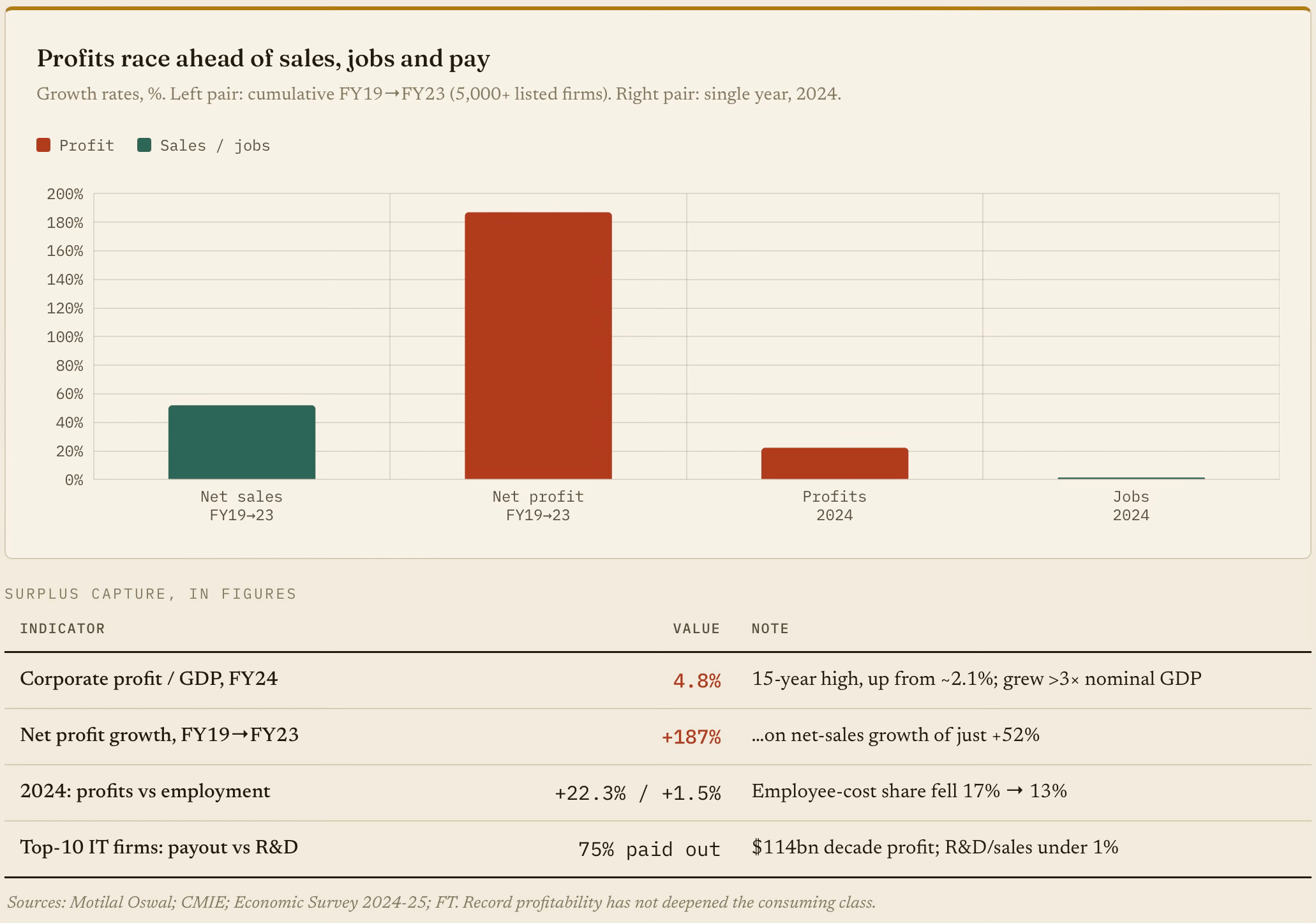
Unfortunately, corporate surpluses are being captured, not recycled into the wages that would create the next tier of consumers. Profits race ahead while sales, jobs and pay lag far behind.
It also does not help that Indian businesses across sectors are averse to spending on R&D and innovation.
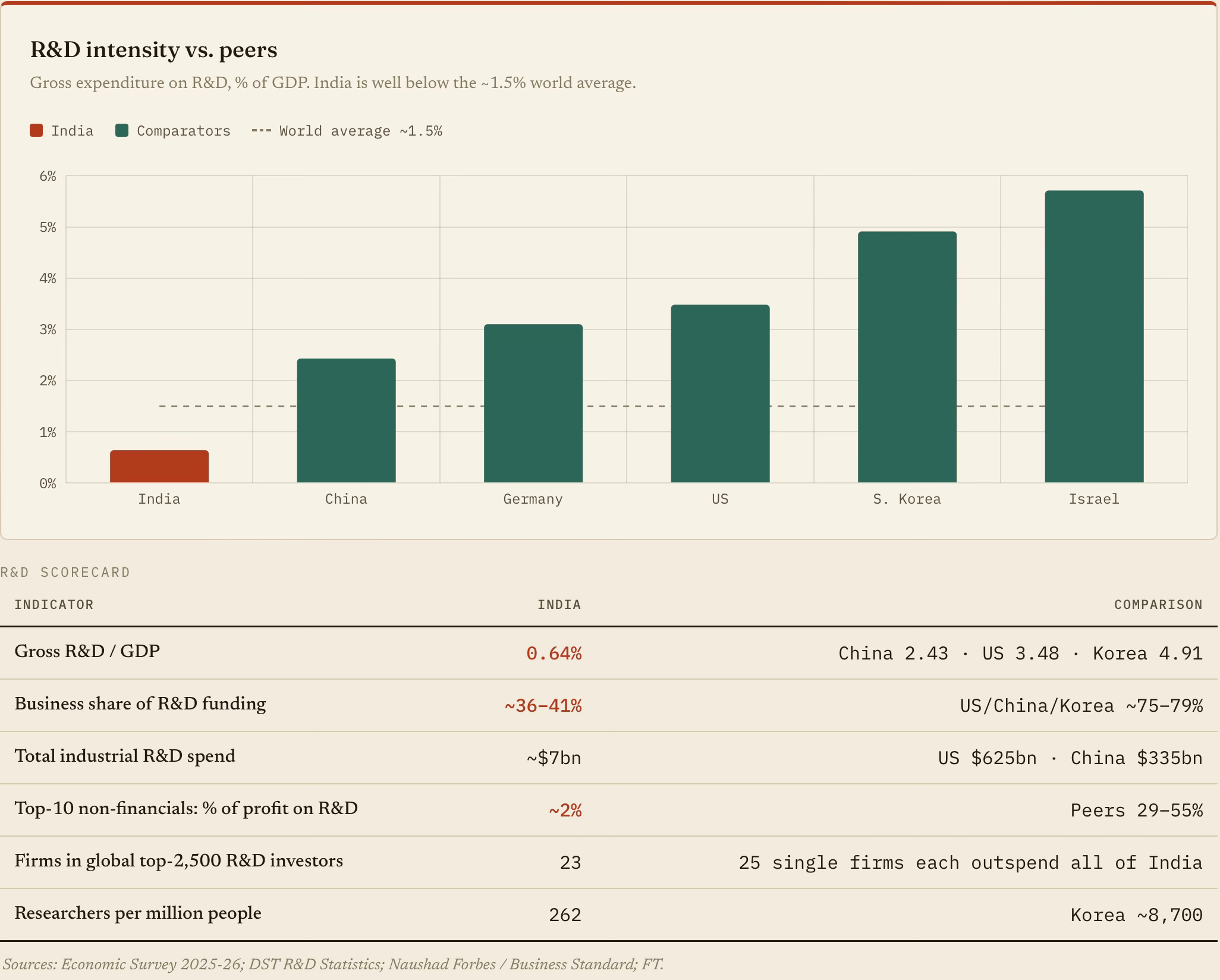
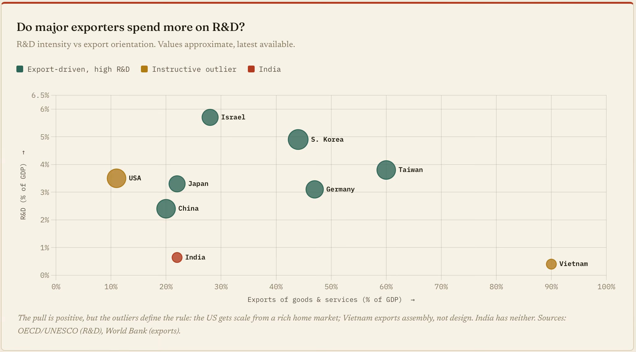
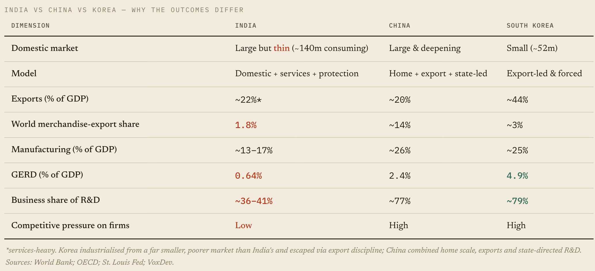
R&D is a fixed cost that only pays off over a large, contestable market. A thin domestic market depresses the return to it, which is why the economies that lead on R&D expenditures are either big-and-rich at home (the US) or export-driven (Korea, Germany, Taiwan). India is neither, and sits alone in the low-R&D corner.
This is an instructive comparison of India with China and South Korea.
The main takeaway is that India’s existing consumption class, confined to just 10% of the households, is too narrow to sustain high growth rates for long periods. It requires considerable broadening. But broad basing economic growth requires access to good jobs, a daunting task given that the gig economy is the biggest source of job creation and elsewhere it is mainly contractual jobs. Worsening matters is the reluctance of the private sector to invest or innovate.